gdistance: Distances and Routes on Geographical Grids
Jacob van Etten
Systems Transformation, Bioversity International, Montpellier, FranceSource:
vignettes/Overview.Rmd
Overview.RmdSummary
The R package gdistance provides
classes and functions to calculate various distance measures and routes
in heterogeneous geographic spaces represented as grids. Least-cost
distances as well as more complex distances based on (constrained)
random walks can be calculated. Also the corresponding routes or
probabilities of passing each cell can be determined. The package
implements classes to store the data about the probability or cost of
transitioning from one cell to another on a grid in a memory-efficient
sparse format. These classes make it possible to manipulate the values
of cell-to-cell movement directly, which offers flexibility and the
possibility to use asymmetric values. The novel distances implemented in
the package are used in geographical genetics (applying circuit theory),
but may also have applications in other fields of geospatial
analysis.
This vignette was published as an article in the Journal of Statistical Software:
van Etten, Jacob. (2017). “R Package gdistance: Distances and Routes on Geographical Grids.” Journal of Statistical Software 76 (13): 1–21. https://doi.org/10.18637/jss.v076.i13.
Introduction: the crow, the wolf, and the drunkard
This vignette describes gdistance, a package written for use in the
R environment (R Core Team
2016). It provides functionality to calculate various distance
measures and routes in heterogeneous geographic spaces represented as
grids. Distance is fundamental to geospatial analysis (Tobler 1970). It is closely related to the
concept of route. For example, take the great-circle distance, the most
commonly used geographic distance measure. This distance represents the
shortest line between two points, taking into account the curvature of
the earth. Implicit in this distance measure is a route. The
great-circle distance could be conceived of as the distance measured
along a route of a very efficient traveller who knows where to go and
has no obstacles to deal with. In common language, this is referred to
as distance `as the crow flies’.
Other distance measures also imply a route across geographic space. The least-cost distance is implemented in most GIS software and mimics route finding ‘as the wolf runs’, taking into account obstacles and the local `friction’ of the landscape. Since least-cost distance is affected by the environment, grid-based calculations are necessary. Other grid-based distances have been developed based on the random walk or drunkard’s walk, in which route-finding is a stochastic process.
Package gdistance was designed to determine such grid-based distances and routes and to be used in combination with other packages available within R. The gdistance package is comparable to other software such as ArcGIS Spatial Analyst (McCoy and Johnston 2002), GRASS GIS ( Development Team 2017), and CircuitScape (B. H. McRae et al. 2008). The gdistance package also contains specific functionality for geographical genetic analyses, not found in other software yet. The package implements measures to model dispersal histories first presented by (J. van Etten and Hijmans 2010).
Theory
In gdistance calculations are done in various steps. This can be confusing at first for those who are used to distance and route calculations in GIS software, which are usually done in a single step. However, an important goal of gdistance is to make the calculations of distances and routes more flexible, which also makes the package more complicated to use. Users, therefore, need to have a basic understanding of the theory behind distance and route calculations.
Calculations of distances and routes start with raster data. In geospatial analysis, rasters are rectangular, regular grids that represent continuous data over geographical space. Cells are arranged in rows and columns and each holds a value. A raster is accompanied by metadata that indicate the resolution, extent and other properties.
Distance and route calculations on rasters rely on graph theory. So as a first step, rasters are converted into graphs by connecting cell centres to each other, which become the nodes in the graph. This can be done in various ways, but only three neighbourhood graphs are commonly implemented in distance calculation software (Figure 1).
- Cells can be connected orthogonally to their four immediate neighbours, the von Neumann neighbourhood.
- Cells can be connected with their eight orthogonal and diagonal nearest neighbours, the Moore neighbourhood. The resulting graph is called the king’s graph, because it reflects all the legal movements of the king in chess. This is the most common and often only way to connect grids in GIS software.
- Connecting the cell centres in 16 directions combines king’s and knight’s moves. The function r.cost in the software GRASS ( Development Team 2017) has this as an option, which inspired its implementation in gdistance. The section on distance transforms in (de Smith, Goodchild, and Longley 2009) also discusses 16-cell neighbourhoods. Connecting in 16 directions may increase the accuracy of the calculations.
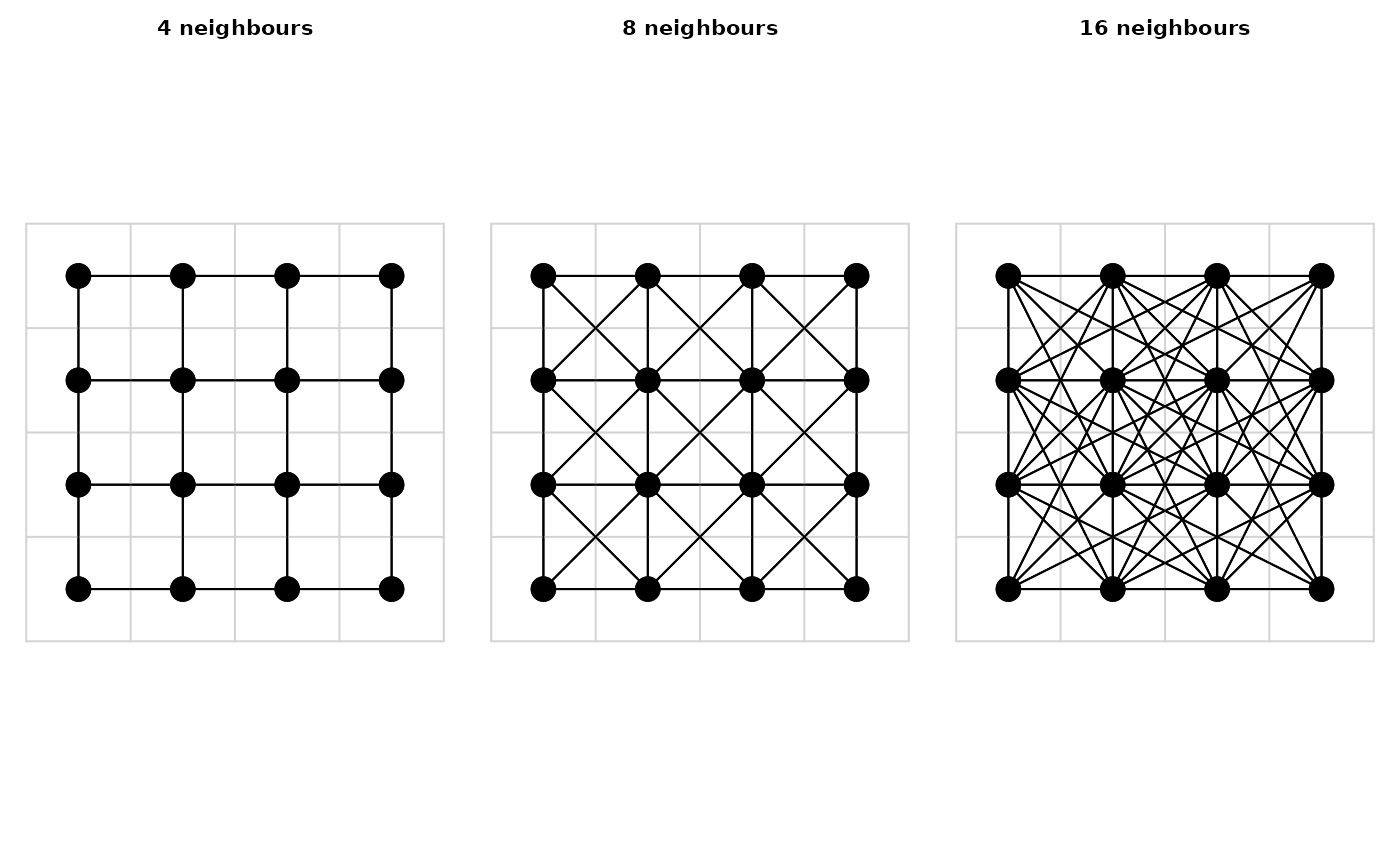
Fig.1 : Three commonly used ways to generate neighbour graphs for distance calculations.
When the raster is converted into a graph, weights are given to each edge (connections between nodes). These weights correspond to different concepts. In most GIS software, distance analyses are done with calculations using cost, friction or resistance values. In graph theory, weights can also correspond to conductance (1/resistance), which is equivalent to permeability (a term used in landscape ecology). The weights can also represent probabilities of transition.
Graphs are mathematically represented as matrices to do calculations. These can include transition probability matrices, adjacency matrices, resistance/conductance matrices, Laplacian matrices, among others. In gdistance, we refer collectively to these matrices to represent graphs as `transition matrices’. These transition matrices are the central object in the package; all distance calculations need one or more transition matrices as an input.
In gdistance, conductance rather than resistance values are expected in the transition matrix. An important advantage of using conductance is that it makes it possible to store values in computer memory very efficiently. Conductance matrices usually contain mainly zeros, because cells are connected only with adjacent cells, and the conductance for direct connections between remote cells is zero. This makes conductance matrices suitable to store in the memory-efficient sparse matrix format. Sparse matrices do not store zero values explicitly in computer memory; they just store the non-zero values and their respective row and column indices and assume that the other values are zero. Sparse matrices do not work for resistance matrices, however, as resistance is infinite (\(\infty\)) between unconnected cells.
The calculation of the edge weights or conductance values is usually based on the values of the pair of grid cells to be connected. These cell values represent a property of the landscape. For instance, from a grid with altitude values, a value for the ease of walking can be calculated for each transition between cells. In gdistance, users define a function \(f(i,j)\) to calculate the transition value for each pair of adjacent cells i and j.
With this approach, it is possible to create asymmetric matrices, in which the conductance from cell i to adjacent cell j is not always the same as the conductance from j back to i. This is relevant, among other things, for modelling travel in hilly terrain, as shown in Example 1 below. On the same slope, a downslope traveler experiences less friction than an upslope traveler. In this case, the function to calculate conductance values is non-commutative: \(f(i,j) \neq f(j,i)\).
A problem that arises in grid-based modelling is the choice of weights that should be given to diagonal edges in proportion to orthogonal ones. For least-cost path distance and routes, this is fairly straightforward: weights are given in proportion to the distances between the cell centres. In a grid in which the orthogonal edges have a length of 1, the diagonal edges are \(\sqrt[]{2}\) long. (B. H. McRae 2006) applies this same idea to random walks. However, as (Birch 2006) explains, for random walks this is generally not the best discrete approximation of the dispersal process in continuous space. Different orthogonal and diagonal weights could be considered based on his analytical results.
For random walks on longitude-latitude grids, there is an additional consideration to be made. Considering the eight neighbouring cells in a Moore’s neighbourhood, the three cells that are located nearer to the equator are larger in area than the three cells that are closer to the nearest pole, as the meridians converge when moving from the equator to either pole. So the cells closer to the poles should have a slightly lower probability of being reached during a random walk from the central cell. More theoretical work is needed to investigate possible solutions to this problem. For projected grids and small areas, we can safely ignore the surface distortion.
When the transition matrix has been constructed, different algorithms to calculate distances and routes are applied.
- The least-cost distance mimics route finding ‘as the wolf runs’, taking into account obstacles and the local ‘friction’ of the landscape. In gdistance the least-cost path between two cells on the grid and the associated distance is obtained with Dijkstra’s algorithm (Dijkstra 1959).
- A second type of route-finding is the random walk, which has no predetermined destination (a ‘drunkard’s walk’). Commute distance represents the random walk commute time, e.g., the average number of edges traversed during a random walk from an starting point on the graph to a destination point and back again to the starting point (Chandra et al. 1996). Resistance distance reflects the average travel cost during this walk (B. H. McRae 2006). When taken on the same graph these two measures differ only in their scaling (Kivimäki, Shimbo, and Saerens 2014). Commute and resistance distances are calculated using the analogy with an electrical circuit see (Doyle and Snell 1984) for an introduction. The algorithm that gdistance uses to calculate commute distances was developed by (Fouss et al. 2007).
- A third type of route-finding is by randomised shortest paths, which are an intermediate form between shortest paths and Brownian random walks, introduced by (Saerens et al. 2009). By setting a parameter, \(\theta\) (theta), in the randomised shortest paths calculation, distances and routes can be made more randomised. A lower value of \(\theta\) means that walkers explore more around the shortest path. When \(\theta\) approaches zero, the randomised shortest paths approach a random walk. (J. van Etten and Hijmans 2010) applied randomised shortest paths in geospatial analysis (and see Example 2 below).
Raster basics
Analyses in gdistance start with one or more
rasters. For this, it relies on another R package,
raster (Hijmans and van Etten
2016). The raster package provides comprehensive
geographical grid functionality. Here, we briefly discuss this package,
referring the reader to the documentation of raster
itself for more information. The following code shows how to create a
raster object.
library("gdistance")
set.seed(123)
r <- raster(ncol = 3, nrow = 3)
r[] <- 1:ncell(r)
r
#> class      : RasterLayer
#> dimensions : 3, 3, 9  (nrow, ncol, ncell)
#> resolution : 120, 60  (x, y)
#> extent     : -180, 180, -90, 90  (xmin, xmax, ymin, ymax)
#> crs        : +proj=longlat +datum=WGS84 +no_defs
#> source     : memory
#> names      : layer
#> values     : 1, 9  (min, max)
The first line loads the package gdistance, which automatically loads the package raster as well. The second line creates a simple raster with 3 columns and 3 rows. The third line assigns the values 1 to 9 as the values of the cells. The resulting object is inspected in the fourth line. As can be seen in the output, the object does not only hold the cell values, but also holds metadata about the geographical properties of the raster.
It can also be seen that this is an object of the class
RasterLayer. This class is for objects that hold only one
layer of grid data. There are other classes which allow more than one
layer of data: RasterStack and RasterBrick.
Collectively, these classes are referred to as Raster*. A
class is a static entity designed to represent objects of a certain type
using ‘slots’, which each hold different information about the object.
Both raster and gdistance use
so-called S4 classes, a formal object-oriented system in R.
An advantage of using classes is that data and metadata stay together
and remain coherent. Consistent use of classes makes it more difficult
to have contradictions in the information about an object. For example,
changing the number of rows of a grid also has an effect on the total
number of cells. Information about these two types of information of the
same object could become contradictory if we were allowed to change one
without adjusting the other. Classes make operations more rigid to avoid
such contradictions. Operations that are geographically incorrect can
also be detected in this way. For example, when the user tries to add
the values of two rasters of different projections, the
raster package will detect the difference and throw an
error.
Classes also make it easier for the users to work with complex data
and functions. Since so much information can be stored in a consistent
way in objects and passed to functions, these functions need fewer
options. Functions can deduce from the class of the object that is given
to it, what it needs to do. The use of classes, if well done, tends to
produce cleaner, more easily readable, and more consistent scripts. One
important thing to know about raster is how grid data
are stored internally in Raster* objects. Consecutive cell
numbers in rasters go from left to right and from top to bottom. The 3 x
3 raster we just created with its cell numbers is shown in Figure 2.
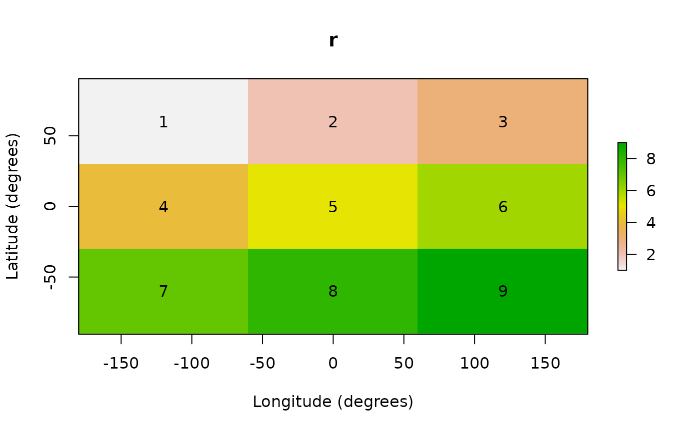
Fig. 2: Lon-lat grid with cell numbers of a 3 × 3 raster
Transition* classes
As explained in Section 2 on the theory behind
gdistance, transition matrices are the backbone of the
package. The key classes in gdistance are
TransitionLayer and TransitionStack. Most
functions in the package have an object of one of these classes as input
or output.
Transition* objects can be constructed from an object of
class Raster*. A Transition* object takes the
necessary geographic references (projection, resolution, extent) from
the original Raster* object. It also contains a matrix
which represents a transition from one cell to another in the grid. Each
row and column in the matrix represents a cell in the original
Raster* object. Row 1 and column 1 in the transition matrix
correspond to cell 1 in the original raster, row 2 and column 2 to cell
2, and so on. For example, the raster we just created would produce a 9
x 9 transition matrix with rows and columns numbered from 1 to 9 (see
Figure 3 below).
The matrix is stored in a sparse format, as discussed in Section 2.
The package gdistance makes use of sparse matrix
classes and methods from the package Matrix, which
gives access to fast procedures implemented in the C
language (Bates and Maechler 2017). The
construction of a Transition* object from a
Raster* object is straightforward. We can define an
arbitrary function to calculate the conductance values from the values
of each pair of cells to be connected.
In the following chunk of code, we use the RasterLayer
that was created above. First, we set all its values to unit. The next
line creates a TransitionLayer, setting the transition
value between each pair of cells to the mean of the two cell values that
are being connected. The directions argument is set to 8,
which connects all cells to their 8 neighbours (Moore
neighbourhood).
r[] <- 1
tr1 <- transition(r, transitionFunction = mean, directions = 8)
#> The extent and CRS indicate this raster is a global lat/lon raster. This means that transitions going off of the East or West edges will 'wrap' to the opposite edge.
#> Global lat/lon rasters are not supported under new optimizations for 4 and 8 directions with custom transition functions. Falling back to old method.
If we inspect the object we created, we see that the resulting
TransitionLayer object retains much information from the
original RasterLayer object.
tr1
#> class      : TransitionLayer
#> dimensions : 3, 3, 9  (nrow, ncol, ncell)
#> resolution : 120, 60  (x, y)
#> extent     : -180, 180, -90, 90  (xmin, xmax, ymin, ymax)
#> crs        : +proj=longlat +datum=WGS84 +no_defs
#> values      : conductance
#> matrix class: dsCMatrix
To illustrate how to create an asymmetric matrix, we first create a
non-commutative distance function, ncdf. We then use this
function as an argument in the function transition. To make
sure that the resulting transition matrix is indeed asymmetric, we set
the symm argument in transition to
FALSE.
r[] <- runif(9)
ncf <- function(x) max(x) - x[1] + x[2]
tr2 <- transition(r, ncf, 4, symm = FALSE)
#> The extent and CRS indicate this raster is a global lat/lon raster. This means that transitions going off of the East or West edges will 'wrap' to the opposite edge.
#> Global lat/lon rasters are not supported under new optimizations for 4 and 8 directions with custom transition functions. Falling back to old method.
tr2
#> class      : TransitionLayer
#> dimensions : 3, 3, 9  (nrow, ncol, ncell)
#> resolution : 120, 60  (x, y)
#> extent     : -180, 180, -90, 90  (xmin, xmax, ymin, ymax)
#> crs        : +proj=longlat +datum=WGS84 +no_defs
#> values      : conductance
#> matrix class: dgCMatrix
Note the difference between tr1 and tr2 in
the slot ‘matrix class’. This slot holds information about the matrix
class as defined in the package Matrix (Bates and Maechler 2017). The class
dsCMatrix is for matrices that are symmetric. The class
dgCMatrix holds an asymmetric matrix.
Different mathematical operations can be done with
Transition* objects. This makes it possible to flexibly
model different components of landscape friction.
tr3 <- tr1 * tr2
tr3 <- tr1 + tr2
tr3 <- tr1 * 3
tr3 <- sqrt(tr1)
Operations with more than one object require that the different objects have the same resolution and extent. Also, it is possible to extract and replace values in the matrix using indices, in a similar way to the use of indices with simple matrices.
tr3[cbind(1:9, 1:9)] <- tr2[cbind(1:9, 1:9)]
tr3[1:9, 1:9] <- tr2[1:9, 1:9]
tr3[1:5, 1:5]
#> 5 x 5 sparse Matrix of class "dgCMatrix"
#>
#> [1,] .         1.2890328 0.5303763 1.4784573 .
#> [2,] 0.2875775 .         0.4089769 .         1.0926294
#> [3,] 0.2875775 1.1676333 .         .         .
#> [4,] 0.2875775 .         .         .         0.9979172
#> [5,] .         0.7883051 .         0.8830174 .
The functions adjacent (from raster)
and adjacencyFromTransition (from
gdistance) can be used to create indices. Example 1
below illustrates this.
Some functions require that Transition* objects do not
contain any isolated ‘clumps’, islands that are not connected to the
rest of the raster cells. This can be avoided when creating
Transition* objects, for instance by giving conductance
values between all adjacent cells a small minimum value. It can be
checked visually if there are any clumps. For the first method, the user
can extract the transition matrix with function
transitionMatrix. This gives a sparse matrix which can be
vizualized with function image. This shows the rows and
columns of the transition matrix and indicates which has a non-zero
value, which represents a connection between cells (Figure 3).
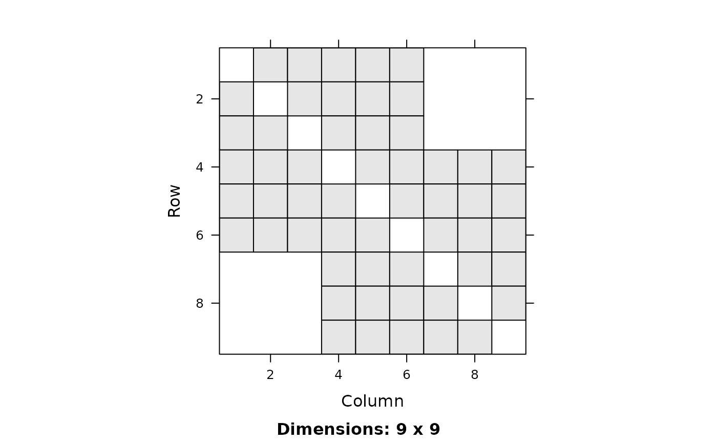
Fig. 3: Visualizing a TransitionLayer with function image
Figure 3 shows which cells are connected to each other. A close observer of Figure 3 may wonder why cell 1 is connected to 5 different cells, as this cell is located in the upper left corner of the original grid. This is explained by the extent of this particular grid. Since it covers the whole world, the outer meridians (180 and -180 degrees) touch each other. The software takes this into account and as a result the cells in the extreme left column are connected to the extreme right column. If the grid does not reach across the globe in longitudinal direction, this does not occur.
Figure 3 shows which cells contain non-zero values, but gives no
further information about levels of conductance. The levels can be
visualized by transforming the transition matrix back into a raster. To
summarize the information in the transition matrix, we can take means or
sums across rows or columns. Users can do this with function
raster. For the different options see
method?raster("TransitionLayer"). The default, shown in
Figure 4, takes the column-wise means of the non-zero values.
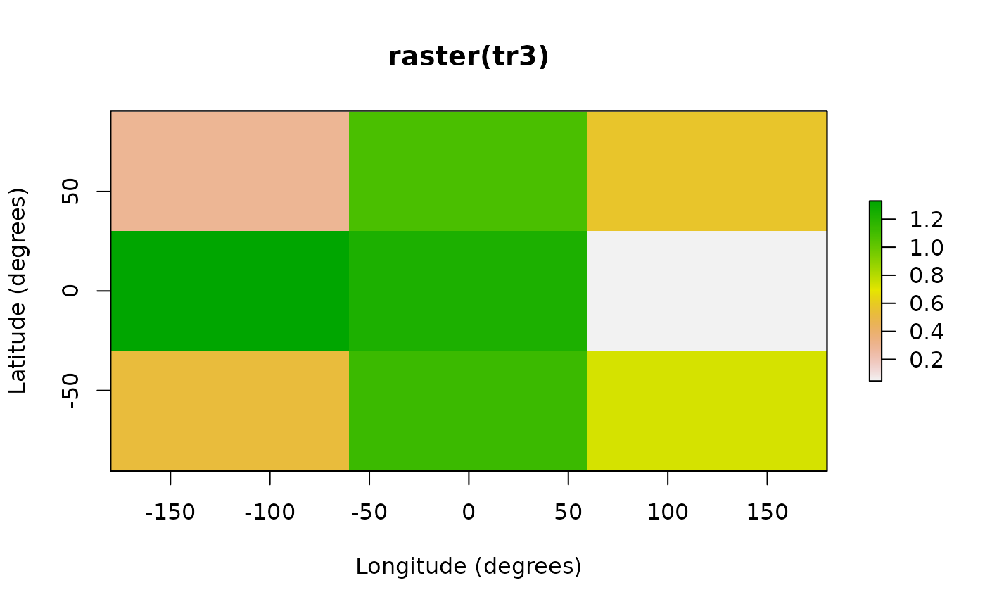
Fig. 4: Visualizing a TransitionLayer using the function raster. The result is a lon-lat grid with the same extent as the original RasterLayer.
Correcting transition matrix values
The function transition calculates transition values
based on the values of adjacent cells in the input raster. However,
diagonal neighbours are more remote from each other than orthogonal
neighbours. Also, on equirectangular (longitude-latitude) grids,
West-East connections are longer at the equator and become shorter
towards the poles, as the meridians approach each other.
Therefore, the values in the matrix need to be corrected for these
two types of distance distortion. Both types of distortion can be
corrected by dividing each conductance matrix value by the distance
between cell centres. This is what function geoCorrection
does when type is set to “c”.
tr1C <- geoCorrection(tr1, type = "c")
tr2C <- geoCorrection(tr2, type = "c")
However, as explained in Section 2 above, for commute distances
(random walks) not only distance distortion plays a role, but also
surface distortion. When type is set to “r” the function
geoCorrection weights the probability of reaching an
adjacent cell in a random walk by simply making it proportional to the
surface covered by the cell. Computationally, the function corrects the
surface distortion by multiplying the North-South transition values with
the cosine of the average latitude of the two cell centres that are
being connected.
r3 <- raster(ncol = 18, nrow = 9)
r3 <- setValues(r3, runif(18 * 9) + 5)

tr3 <- transition(r3, mean, 4)
#> The extent and CRS indicate this raster is a global lat/lon raster. This means that transitions going off of the East or West edges will 'wrap' to the opposite edge.
#> Global lat/lon rasters are not supported under new optimizations for 4 and 8 directions with custom transition functions. Falling back to old method.
tr3C <- geoCorrection(tr3, type = "c", multpl = FALSE, scl = TRUE)
tr3R <- geoCorrection(tr3, type = "r", multpl = FALSE, scl = TRUE)
The argument scl is set to TRUE to scale
the transition values to a reasonable range. If the transition values
are too large, commute distance and randomized shortest path functions
will not work well. No scaling should be done if the user wants to
obtain absolute distance values as output.
In some cases, Transition* objects with equal resolution
and extent need to be corrected many times. For example, determining the
optimal landscape friction weights using a genetic algorithm involves
repeating the same calculations with many transition matrices that only
differ in their values, but not in their resolution or extent (J. van Etten and Hijmans 2010). In this case,
computational effort can be reduced by preparing an object that only
needs to be multiplied with the Transition* object to
produce a corrected version of it.
The following chunk of code is equivalent to the previous one.
CorrMatrix <- geoCorrection(tr3, type = "r", multpl = TRUE, scl = TRUE)
tr3R <- tr3 * CorrMatrix
Object CorrMatrix is only calculated once. It can be
multiplied with Transition* objects, as long as they have
the same extent, resolution, and directions of cell connections. We need
to take special care that the geo-correction multiplication matrix
(CorrMatrix) contains all non-zero values that are present
in the Transition* object with which it will be multiplied
(tr3 in this case).
Calculating distances
After obtaining the geographically corrected Transition*
object, we can calculate distances between points. It is important to
note that all distance functions require a Transition*
object with conductance values, even though distances will be expressed
in 1/conductance (friction or resistance) units (see Section 2
above).
To calculate distances, we need to have the coordinates of point
locations. This is done by creating a two-column matrix of coordinates.
Functions will also accept a SpatialPoints object or, if
there is only one point, a vector of length two.
Calculating a distance matrix is straightforward now.
costDistance(tr3C, sP)
#>           1         2
#> 2 0.8842550
#> 3 0.9508077 1.5139996
commuteDistance(tr3R, sP)
#>           1         2
#> 2  998.0584
#> 3  980.4971 1085.3238
rSPDistance(tr3R, sP, sP, theta = 1e-12, totalNet = "total")
#>          [,1]     [,2]     [,3]
#> [1,]  0.00000 57.91140 56.75376
#> [2,] 56.62602  0.00000 62.12604
#> [3,] 55.76832 62.42598  0.00000
The costDistance function relies on the package
igraph (Csardi and Nepusz
2006) for the underlying calculation. It gives a symmetric or
asymmetric distance matrix, depending on the
TransitionLayer that is used as input.
Commute distance is the number of cells traversed during a random walk from a cell \(i\) on the grid to a cell \(j\) and back to \(i\) (Chandra et al. 1996).
rSPDistance gives the cost incurred during the same walk
(\(\theta\) approaches zero, so this is
the cost incurred during a random walk, see Section 2). To obtain the
commute costs we sum the corresponding off-diagonal elements: \(d_{ij} + d_{ji}\). This is the distance of
a commute from \(i\) to \(j\) and back from \(j\) to \(i\).
In this case, the commute costs (resistance) are close to the commute
distances (number of steps). This is because the
TransitionLayer object has been scaled, so that transition
costs are close to unit for each step and the total number of steps and
the total distance are of the same order of magnitude.
Dispersal paths
To determine dispersal paths of a (constrained) random walk, we use
the function passage. This function can be used for both
random walks and randomised shortest paths. The function calculates the
average number of passages through cells or connections between cells
before arriving in the destination cell. Either the total or net number
of passages can be calculated. The net number of passages is the number
of passages that are not reciprocated by a passage in the opposite
direction. In other words, this is the probability of the “last forward”
passage going through a cell-to-cell connection (B. H. McRae et al. 2008).
Figure 5 shows the net passages through each cell, assuming randomised shortest paths with the parameter \(\theta\) set to 3.
origin <- SpatialPoints(cbind(0, 0))
rSPraster <- passage(tr3C, origin, sP[1, ], theta = 3)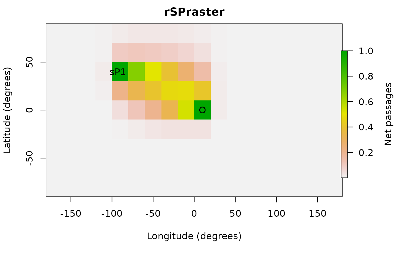
Fig. 5. Net passages from origin O to destination sP1.
Path overlap and non-overlap
One of the specific uses for which package gdistance was created, is to look at dispersal trajectories of organisms that expand their range coming from a single source (J. van Etten and Hijmans 2010). The degree of coincidence of two trajectories can be determined by calculating the minimum of the net passages of the two trajectories. With a formula presented in (J. van Etten and Hijmans 2010), we can approximate the non-overlapping part of the trajectory. This is done in the following code.
r1 <- passage(tr3C, origin, sP[1, ], theta = 1)
r2 <- passage(tr3C, origin, sP[2, ], theta = 1)
rJoint <- min(r1, r2)
rDiv <- max(max(r1, r2) * (1 - min(r1, r2)) - min(r1, r2), 0)
The first two lines create two different trajectories, both coming
from the same point of origin (O) and going to different end
destinations (referred to as sP1 and sP2 in the following). The third
line obtains the minimum probability as a measure of the overlap between
the two trajectories. The resulting raster rJoint is
visualized in Figure 6. The fourth line calculates the non-overlapping
part of the trajectories with a more complicated formula. The result,
rDiv, is shown in Figure 7.
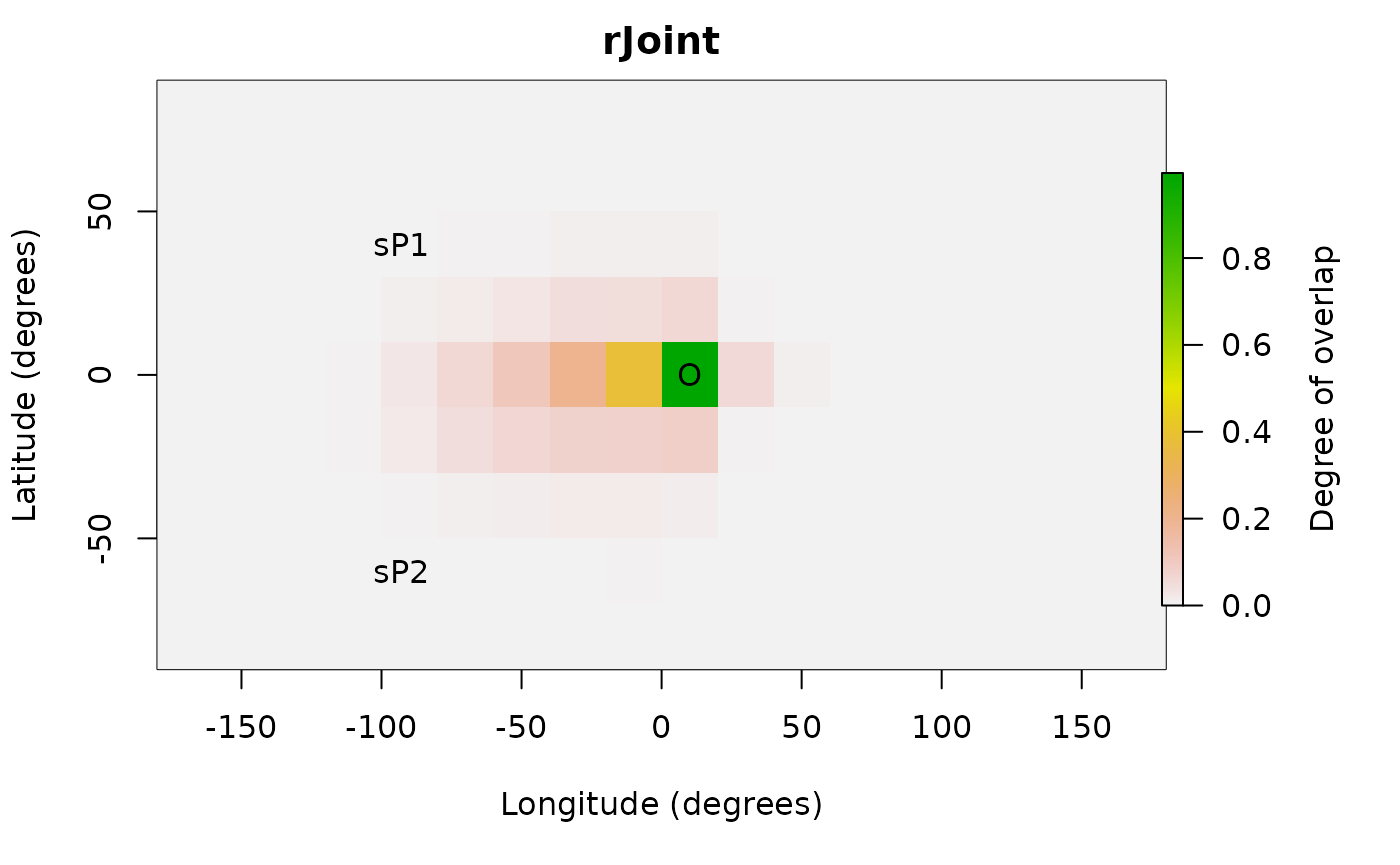
Fig. 6. Overlapping part of the two routes from origin O to sP1 and sP2 respectively.
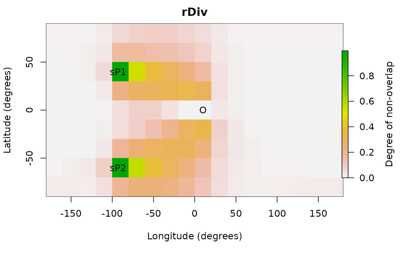
Fig. 7. Non-overlapping part of the two routes from origin O to sP1 and sP2 respectively.
With the function pathInc we can calculate measures of
path overlap and non-overlap for a large number of points. These
measures can be used to predict patterns of diversity if these are due
to dispersal from a single common source. If the argument
type contains two or more elements, the result is a list of
distances matrices. The default for type is to calculate
joint and divergent length of the dispersal paths.
pathInc(tr3C, origin, sP)
#> $function1layer1
#>          1        2
#> 2 2.363770
#> 3 2.318019 2.100372
#>
#> $function2layer1
#>          1        2
#> 2 2.255957
#> 3 2.397766 2.802147
Example 1: Hiking around Maunga Whau
The previous examples were theoretical, based on randomly generated values. More realistic examples serve to illustrate the various uses that can be given to this package.
Determining the fastest route between two points in complex terrain is useful for hikers. Tobler’s Hiking Function provides a rough estimate of the maximum hiking speed (\(s\)) given the slope of the terrain (\(m\)) (Tobler 1993). The maximum speed of off-path hiking (in m/s) is:
\[ s = 6 e^{-3.5 |m + 0.05|} \]
Note that the function is not symmetric around 0 (see Figure 8). Hikers walk fastest on gently downward slopes (\(m = -0.05\)), where they can walk faster than on flat terrain (\(m = 0\)).

Fig. 8. Tobler’s Hiking Function.
We use the Hiking Function to determine the shortest path to hike
around the volcano Maunga Whau (Auckland, New Zealand). First, we read
in the altitude data for the volcano. This is the R base
dataset (see ?volcano).
r <- raster(system.file("external/maungawhau.grd", package = "gdistance"))The Hiking Function requires the slope (\(m\)) as input, which can be calculated from the altitude (\(z\)) and distance between cell centres (\(d\)).
\[ m_{ij} = (z_j - z_i) / d_{ij} \]
The units of altitude and distance should be identical. Here, we use
meters for both. First, we calculate the altitudinal differences between
cells. Then we use the geoCorrection function to divide by
the distance between cells.
altDiff <- function(x) { x[2] - x[1] }
hd <- transition(r, altDiff, 8, symm = FALSE)
#> Warning in .TfromR_new(x, transitionFunction, directions, symm): transition
#> function gives negative values
slope <- geoCorrection(hd)The transition function throws a warning, because a
matrix with negative values cannot be used directly in distance
calculations. Here this warning can be safely ignored, however, as the
negative values are only present in intermediate steps. Subsequently, we
calculate the speed. We need to exercise special care, because the
matrix values between non-adjacent cells is 0, but the slope between
these cells is not 0! Therefore, we need to restrict the calculation to
adjacent cells. We do this by creating an index for adjacent cells
(adj) with the function adjacent.
Using this index, we extract and replace adjacent cells, without touching the other values.
adj <- adjacent(r, cells = 1:ncell(r), pairs = TRUE, directions = 8)
speed <- slope
speed[adj] <- 6 * exp(-3.5 * abs(slope[adj] + 0.05))
Now we have calculated the speed of movement between adjacent cells.
We are close to having the final conductance values. Attainable speed is
a measure of the ease of crossing from one cell to another on the grid.
However, we also need to take into account the distance between cell
centres. Travelling with the same speed, a diagonal connection between
cells takes longer to cross than a straight connection. Therefore, we
use the function geoCorrection again.
Conductance <- geoCorrection(speed) This gives our final ‘conductance’ values. What do these values mean?
The function geoCorrection divides the values in the matrix
between the distance between cell centres. So, with our last command we
calculated conductance (\(C\)) as
follows:
\[ C = s / d \]
This looks a lot like a measure that we are more familiar with, travel time (\(t\)):
\[ t = d / s \]
In fact, the conductance values we have calculated are the reciprocal of travel time (\(1/t\)).
\[ 1 / t = s / d = C \]
Maximizing the reciprocal of travel time is exactly equivalent to minimizing travel time. Distances calculated with this conductance matrix represent travel time according to the Hiking Function.
In the next step, we define two coordinates, A and B, and determine the paths between them. We test if the quickest path from A to B is the same as the quickest path from B back to A. The following code creates the shortest paths.
A <- c(2667670, 6479000)
B <- c(2667800, 6479400)
AtoB <- shortestPath(Conductance, A, B, output = "SpatialLines")
BtoA <- shortestPath(Conductance, B, A, output = "SpatialLines")
And this code reproduces Figure 9.
plot(r, xlab = "x coordinate (m)", ylab = "y coordinate (m)", legend.lab = "Altitude (masl)")
lines(AtoB, col = "red", lwd = 2)
lines(BtoA, col = "blue")
text(A[1] - 10, A[2] - 10, "A")
text(B[1] + 10, B[2] + 10, "B")
A small part of the A-B (red) and B-A (blue) lines in Figure 9 do not overlap. This is a consequence of the asymmetry of the Hiking Function.
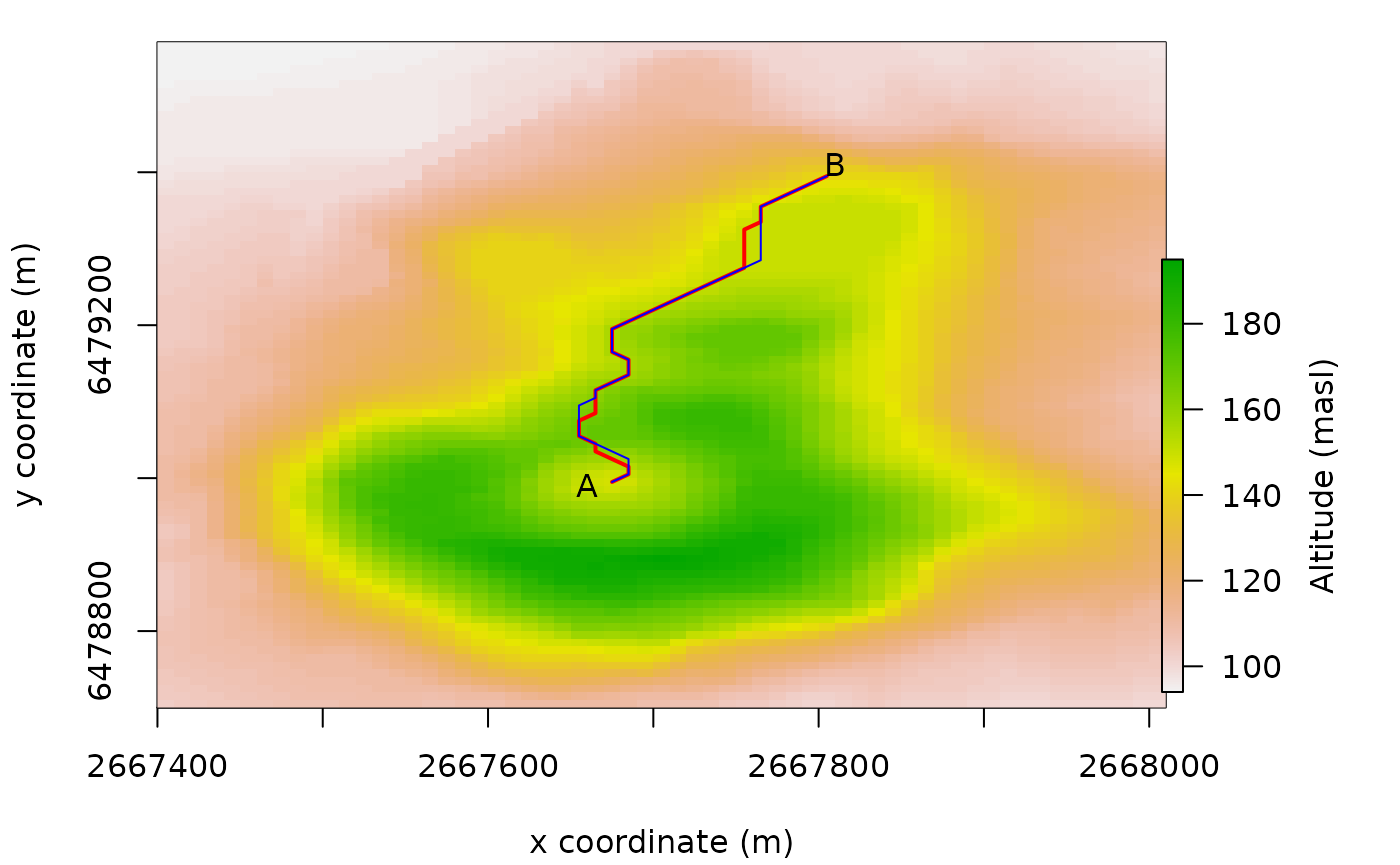
Fig. 9. Quickest hiking routes on Maunga Whau between A and B (A to B is red, B to A is blue). (Coordinate system is the New Zealand Map Grid.)
Example 2: Geographical genetics
A correlation between genetic differentiation and geographic distance of individuals and populations is expected due to a mechanism known as isolation by distance (Wright 1943). This correlation is expected when random, symmetric dispersal occurs in homogeneous geographic spaces. For random dispersal in heterogeneous landscapes, recent work has shown that genetic differentiation correlates with the resistance distance between their locations (B. H. McRae 2006). In this section, we look at human genetic diversity in Europe, using the data presented by (Balaresque et al. 2010).
First, we read in the data: a map of Europe, the coordinates of the
populations (see Figure 10) and mutual genetic distances (see
?genDist for more information on these data).
Europe <- raster(system.file("external/Europe.grd", package = "gdistance"))

data(genDist)
data(popCoord)

pC <- as.matrix(popCoord[c("x", "y")])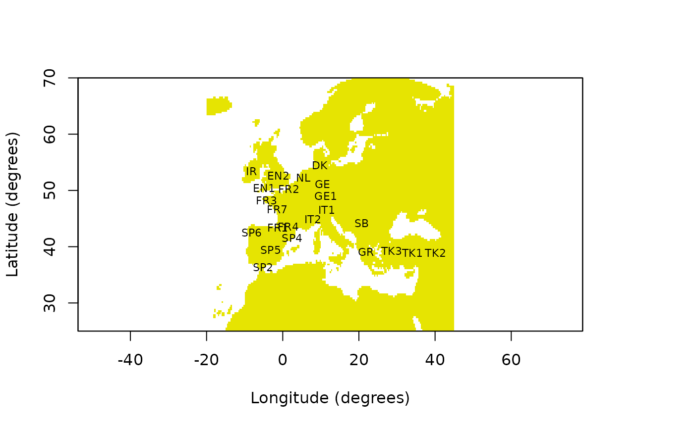
Fig. 10. Map of genotyped populations.
Then we create three geographical distance matrices. The first corresponds to the great-circle distance between populations. The second is the least-cost distance between locations. Travel is restricted to the land mass. The third is the commute distance (using the same conductance matrix), which is related to effective resistance between points if we conceive of the grid as an electrical circuit (Chandra et al. 1996; B. H. McRae 2006).
geoDist <- pointDistance(pC, longlat = TRUE)
geoDist <- as.dist(geoDist)
Europe <- aggregate(Europe, 3)

# Keep only the largest "clump" and remove patches that cannot be reached.
# Having disconnected patches might sometimes cause issues with some of the
# linear algebra calculations.
# Note that this clump code is not robust to other rasters that will need to identify
# the correct clump number
clumps = raster::clump(Europe, directions = 8)
clumps[clumps[] != 1] <- NA
Europe = Europe * clumps

tr <- transition(Europe, mean, directions = 8)
trC <- geoCorrection(tr, "c", scl = TRUE)
trR <- geoCorrection(tr, "r", scl = TRUE)

cosDist <- costDistance(trC, pC)
resDist <- commuteDistance(trR, pC)

cor(genDist, geoDist)
#> [1] 0.5964302
cor(genDist, cosDist)
#> [1] 0.6055185
cor(genDist, resDist)
#> [1] 0.21269
Among the distance measures evaluated until now, the great-circle distance between points turns out to be the best predictor of genetic distance. The other distance measures incorporate more information about the geographic space in which geneflow takes place, but do not improve the prediction. It follows that prehistoric people in Europe did not move like wolves (least-cost distance) or drunkards (commute or resistance distance), but rather like crows (great-circle distance).
An important assumption behind these distance measures, however, is that dispersal is symmetric. This is often not the case. For example, diffusion from a single origin (Africa) explains much of the current geographical patterns of human genetic diversity (Ramachandran et al. 2005). As a result, the mutual genetic distance between a pair of humans from different parts from the globe depends on the extent they share their prehistoric migration history. Within Europe, genetic diversity is often thought to be a result of the migration of early Neolithic farmers from Anatolia (now part of modern Turkey) to the west.
How well does a geographic wave of expansion from Anatolia explain
the spatial pattern? The function pathInc calculates the
overlap (and non-overlap) of dispersal paths from a common origin on the
grid as a distance measure between points.
origin <- unlist(popCoord[22, c("x", "y")])
pI <- pathInc(trC, origin = origin, from = pC, functions = list(overlap))
cor(genDist, pI[[1]])
#> [1] -0.7332525
At least at first sight, the overlap of dispersal routes explains the spatial pattern better than any of the previous measures. The negative sign of the last correlation coefficient was expected, as more overlap in routes is associated with lower genetic distance. Additional work would be needed to improve predictions and compare the different models more rigorously.
Future work
Improvements of gdistance and methodological
refinements are expected in various areas. * All measures based on
random walks depend critically on solving sparse linear systems. This is
the most time-consuming part of the calculations. Faster libraries could
improve the gdistance package if they become available
in R in the future. * Research on distances in graph theory
is a very dynamic field in the computational sciences. New measures and
algorithms could be added to gdistance when they become
available. * More research on the consequences of connecting grids in
different ways is necessary, as indicated in Section 2. This should
bring more precision to random walk calculations in geospatial analysis.
Comparing the results of grid-based calculations to continuous space
simulations or analytical solutions would be the way forward (Birch 2006).
Acknowledgements
This research is supported by CGIAR Fund Donors. Work on the gdistance package started during the project “Collective Action for the Rehabilitation of Global Public Goods in the CGIAR Genetic Resources System: Phase 2” (2007-2010), under the guidance of Dr Robert Hijmans. Finalizing the package was undertaken as part of the CGIAR Research Program on Climate Change, Agriculture and Food Security (CCAFS), which is a strategic partnership of CGIAR and Future Earth. The views expressed in this document cannot be taken to reflect the official opinions of CGIAR or Future Earth.